
Exploring the Hurst Exponent
Written by Xiaoxue (Rachel) Xiong, Quantitative Trading Intern
Navigating chaos: Unraveling digital asset dynamics using the Hurst exponent
Aug 22, 2023“The brain highlights what it imagines as patterns; it disregards contradictory information. Human nature yearns to see order and hierarchy in the world. It will invent it where it cannot find it."
– In Memory of the late Benoît B. Mandelbrot, The (Mis)Behavior of Markets
The efficient market hypothesis (EMH) states that market returns are the result of new information entering the marketplace, thereby rendering historical price patterns that are irrelevant for future performance. The EMH basically invalidates the efforts of technical analysis that aim to predict prices by solely looking at historical price patterns. In addition, the EMH implies that market returns are random. Both empirically and theoretically, the EMH holds very well. Empirically, there has not been much evidence that market returns can be predicted by only studying observed price patterns. On the theoretical front, laws of statistics imply random returns – if there are many independent events that drive the market, returns would be random.
The existence of predictable momentum and reversion patterns of market prices would contradict the EMH and require additional models to explain them. Here we show that markets are not always efficient and that in the current high volatility environment, behavioral and structural effects (e.g., overreaction to insignificant news) can lead to persistent patterns of momentum and reversion. We apply the Hurst exponent in quantitative trading to identify if a given time series is trending, mean-reverting, or simply a random walk, rather than manually reviewing all stocks to detect trending patterns.
Introducing the Hurst Exponent
Many standard stationary stochastic processes assumed in EMH suggest that the effect of each data point decays so fast that it rapidly becomes indistinguishable from noise. However, in many fields, strong evidence of a long memory phenomenon exists, implying there is non-negligible dependence between the present and all points in the past. Long memory time series have been a popular area of research in economics, climate trends, earthquake modeling, finance, statistics, and others. It was first observed by the hydrologist Harold Edwin Hurst when analyzing the minimal water flow of the Nile River while planning the Aswan Dam. [1] [2]
For thousands of years, the Nile had helped sustain civilizations, yet its regular floods and irregular flows were a severe impediment to development. Harold Edwin Hurst devised a method of water control by taking a holistic view of the Nile basin, from its sources in the African Great Lakes and Ethiopian plains, to the grand delta on the Mediterranean. He examined 690 different time series, covering 75 different geophysical phenomena that spanned a wide range of quantities, including river levels, rainfall, temperature, mud sediment thickness, and sunspots. He discovered a persistent statistical behavior in a study of water flows. Hurst’s work motivated the late Benoît Mandelbrot to develop current long memory theories and applications, and he extended the concept to fractal theory.[3]
Exhibit 1: Three Faces of Hurst Exponent


The concept of the Hurst exponent delves into the notion of fractional dimension, a time series exhibiting a pronounced trend where price returns consistently move in one direction. Such time series possesses a fractional dimension of 1, i.e., a perfectly straight line. Conversely, a time series marked by rapid oscillations and sharp reversals, covering a broad spectrum of values on a chart, has a fractional dimension of 2. To distinguish between trending and reverting behavior, practitioners often focus on the Hurst exponent, which is determined by subtracting the fractional dimension from 2.
To summarize, we classify a Hurst exponent ranging from 0 to 1 into three categories:
Hurst exponent < 0.5: An entirely mean-reverting series, characterized by pronounced reversals, holds a fractional dimension of 2 and an associated Hurst Exponent of 0. If the Hurst exponent is less than 0.5, the time series is considered to exhibit a mean-reverting behavior.
Hurst exponent = 0.5: Complete randomness has a fractional dimension of 1.5, translating to a Hurst exponent of 0.5, indicating that the time series has no memory or autocorrelation.
Hurst exponent > 0.5: In a perfectly trending series, the fractional dimension equates to 1, resulting in a Hurst exponent of 1. If the Hurst exponent is greater than 0.5, the time series is considered to have a persistent or trending behavior.
For additional details of Hurst exponent calculation please see Technical Appendix below.
Fractal Behavior of Digital Assets
Exhibit 2 shows the Detrended Fluctuation Analysis (DFA) Hurst exponents for USD pairs of bitcoin, ether, Binance coin, and EUR, using a sliding window of 500 days.
Exhibit 2: Hurst Exponent of Selected Assets
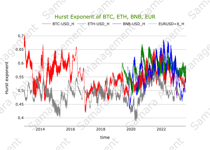
The first observation is that the Hurst exponents are noisy over time and non-stationary. Here, we use EUR-USD (gray) as the benchmark asset for our analysis. EUR-USD is one of the most competitive markets in the world, and as such, its price difference behaves as a random process with the Hurst exponent closely oscillating around 0.5.
The following summarizes our observations and insights:
Bitcoin (red): Prior to 2017 bull market, institutional participation in the bitcoin market was relatively weak, and bitcoin time series had shown a persistently high Hurst exponent of over 0.6. During the bull market of 2017-2018, bitcoin markets became competitive and more efficient as the Hurst exponent stayed around 0.5. The 2020 bull market cycle was characterized by great retail participation, which resulted in strong interest and momentum in the market, with the Hurst exponent reaching 0.65. Post-FTX, bitcoin lost momentum and returned to non-trend regime with the Hurst exponent oscillating around 0.55. Overall, the bitcoin market has improved in efficiency and tends to follow EMH, especially in recent years.
Ether (green): As a mega-name in digital asset industry, ether traces the behavior of bitcoin. Due to less institutional participation, the Hurst exponents of ether tend to be more zig-zagged, with more pronounced regime changes between trending and non-trending market phases. Ether’s price benefited from the DeFi Summer in 2020 and The Merge in 2022, characterized by higher Hurst exponents (0.65). Currently, just like bitcoin, ether is in a non-trending phase.
Binance Coin (blue): The Binance platform token benefited from aggressive marketing campaigns and a Covid-19-led bull market. It is currently non-trending.
From the above analysis of the Hurst exponents, we can see that herd behavior is prevalent in a cryptocurrency time series. This implies that series volatility that tends to grow will grow faster over time if the index is greater than 0.5.
Exhibit 3 investigates the stationary of the rescaled range (R/S) Hurst exponents over 30-, 60-, and 90-day sliding windows.
Exhibit 3: Bitcoin Hurst Exponent at Daily Price Resolution

Contrasting to Exhibit 2, which used a 500-day sliding window, Exhibit 3 shows a strong lagging and averaging effect in the Hurst exponents for bitcoin. At the 30-day sliding window, bitcoin has shown temporary spikes of trending behavior, sometimes exceeding a Hurst exponent of 1. Using a short rolling window will lead to more periods of trending markets, but it will also yield noisier results.
The EMH suggests that prices only move when new information is received. When this happens, the financial markets are temporarily pushed out of equilibrium, causing the market participants to start adjusting their positions. However, it is highly unlikely that market prices absorb news as quickly as implied by the EMH. One reason for this is the fact that markets are non-homogeneous, with market participants having various objectives, time horizons, and constraints. For instance, market makers typically rebalance positions immediately, whereas retail investors typically respond much slower. The lag between an individual news flash and the time at which the position is changed can be substantial for these types of investors.
Exhibit 4: Bitcoin Hurst Exponent at 10 Second Price Resolution

Exhibit 4 shows the Hurst exponents for bitcoin at a high time resolution by using 10-second mid-price snapshots. We observe that the Hurst exponent consistently exceeds 0.7. Such fractal behavior patterns make statistical arbitrage possible, exploiting statistical market properties and inefficiencies on short time scales.
Trading with the Hurst Exponent
A naïve way to implement the mean-reversion strategy would be to buy the market at the close if it is down for the day or sell it at the close if the market is up for the day. Volatility also helps the strategy, as high volatility usually results in lower autocorrelations and provides higher absolute daily returns. However, the Hurst Exponent lacks inherent directional information within its signal and is used in combination with other trading indicators. The Hurst exponent remains a potent instrument to detect trends and optimize trading strategies for a specific epoch or time resolution.
Let’s review a few applications of Hurst exponents in quantitative trading.
Regime Switch Filter
The role of a regime filter resembles that of a traffic control officer overseeing passage on a single-lane bridge. Movement across the bridge is conditional on meeting specific criteria; if these conditions are not met, traversal is restricted. A Hurst exponent exceeding 0.5 signifies a trending behavior of asset price. Notably, instances of positive returns are often succeeded by further positive returns, and conversely for negative returns. Extensive empirical research suggests that such price behavior is attributable to autocorrelation, the correlation of a variable with its own lagged values. Positive autocorrelation implies that positive returns at a certain time are correlated with positive returns in subsequent periods. This phenomenon could arise due to underlying factors like market momentum, investor behavior, or news impact.
We can use the Hurst exponent as a regime filter to segment trending versus non-trending market and optimize the trading strategy. Specifically, traders can search for a Hurst exponent level that increases the percentage of winning trades, reducing transaction costs and improving equity curve.
Position Sizing
Pyramiding is a strategy where investors add to their position in a winning trade as it moves in their favor. It is a way of leveraging profits to potentially increase gains over time. However, pyramiding also comes with increased risk, as the positions become larger with more capital at stake.
The Hurst exponent can act as an objective tool for determining when to pyramid and when to take profits. The Hurst exponent crossing above a certain threshold is a signal to add new positions; the Hurst exponent crossing below a certain threshold is a signal to reduce or exit positions. In combination with a dynamic stop-loss strategy, investors can use the Hurst exponent to optimize profit and reduce risk in a systematic fashion.
A Powerful Analytics Tool
The Hurst exponent is a powerful tool in financial time series analysis, shedding light on the intricate behaviors of markets. Through its nuanced calculation and interpretation, it allows us to decode the underlying dynamics of trends, mean-reversion, and persistent correlations. The Hurst exponent provides a quantitative measure to discern when markets deviate from randomness. Its applications prove to be invaluable in constructing and fine-tuning trading strategies. By leveraging the insights offered by the Hurst exponent, traders can navigate the shifting currents of financial markets and adjust their trading decisions accordingly.
The Hurst exponent is extremely sensitive to the time resolution of time series. Given the dynamic nature of financial market, we need to apply this tool judiciously and in conjunction with other indicators.
The Hurst exponent offers a continuous thread of understanding, a bridge between the intricate patterns woven by human behavior and the apparent randomness of market movements. Investors and traders can navigate the complex interplay of order and chaos, especially in nascent markets like digital assets. Samara Alpha Management aims to strategically capitalize on return abnormalities in these markets, arising as a result of imbalances in market structures and investor behaviors.
Technical Appendix
Method Ⅰ:
The most straightforward approach is to estimate the diffusive behavior by analyzing the variance of logarithmic price values. The steps are below:
Step 1: Apply the natural logarithm to the time series of prices, denoted as $S$. $$\mathrm{x_t} = log {(S_t)}$$ Step 2: Calculate the variance for lag $\tau$. $$\mathrm{Var}(\tau) = |X_{t+\tau} - X_t|^2$$ Step 3: Estimate $\mathrm{Var}(\tau) \sim \tau^{2H}$, where $H$ stands for the Hurst Exponent.
Method Ⅱ:
Another approach to calculate the Hurst Exponent is utilizing rescaled range $(R/S)$ analysis as devised by Harold Edwin Hurst. In this method, the Hurst Exponent is defined as follows: $$E\left[\frac{R(n)}{S(n)}\right] = Cn^H \text{ as } n \to \infty$$ Where:
· $R(n)$ is the range of the first $n$ cumulative deviations from the mean.
· $S(n)$ is the series(sum) of the first $n$ standard deviations.
· $n$ is the time span of the observation (number of data points in a time series).
· $C$ is a constant.
In this method, we first need to estimate the dependence of the rescaled range on the time span $n$ of observation. This involves partitioning a time series with a total length of $N$ into various shorter segments with lengths of $n = N, \frac{N}{2}, \frac{N}{4}$, and so on. Subsequently, the average rescaled range is computed for each of these n values. For a partial time series of length $n$, $X_1, X_2, X_3, \ldots, X_n$, the rescaled range is calculated as follows:
1. Calculate the mean.$$m = \frac{1}{n} \sum_{i=1}^{n} X_i$$ 2. Generate a mean-adjusted series.$$Y_t = X_t - m \quad \text{for } t = 1, 2, \ldots, n$$ 3. Calculate the cumulative deviate series Z. $$Z_t = \sum_{i=1}^{t} Y_i \quad \text{for } t = 1, 2, \ldots, n$$ 4. Compute the range R. $$R(n) = \max(Z_1, Z_2, \ldots, Z_n) - \min(Z_1, Z_2, \ldots, Z_n)$$ 5. Calculate the standard deviation S. $$S(n) = \sqrt{\frac{1}{n}} \sum_{i=1}^{n} (X_i - m)^2$$ 6. Calculate the rescaled range $R(n)/S(n)$ and average over all the partial time series of length $n$.
The Hurst exponent is estimated by fitting the power law.$$E\left[\frac{R(n)}{S(n)}\right] = Cn^H$$
Method Ⅲ
The last approach is the Detrended Fluctuation Analysis (DFA) method. Given the stochastic time series $y(t)$, for $t = 1, 2, \ldots, M$. There are several steps to calculate the Hurst Exponent:
Step 1: Calculate the mean $\bar{y}$ of time series $y(t)$.
Step 2: Calculate integrated time series $x(i)$.$$x(i) = \sum_{i=1}^{t} (y(t) - \bar{y})$$
Step 3: Divide $x(i)$ into $M/m$ non overlapping subsamples. Within each subsample, compute the least squares straight-line fit $x_{\text{pol}}(i, m)$.
Step 4: Compute the fluctuation function.$$F(m) = \sqrt{\frac{1}{M} \sum_{i=1}^{M} (x(i) - x_{\text{pol}}(i, m))^2}$$
Step 5: The fluctuation function $F(m)$ behaves as a power-law of $m$, $F(m)$ $\alpha$ $m^H$. So calculate the Hurst Exponent by regressing $\ln(F(m))$ onto $\ln(m)$.
Contributed by Xiaoxue (Rachel) Xiong – Quantitative Trading Intern
A dedicated Quantitative Researcher with a robust academic background in statistics and machine learning, Xiaoxue is currently pursuing her Master of Arts in Statistics at Columbia University while working as a quantitative researcher at Samara Alpha Management. She specializes in applying data-driven methodologies in financial analysis, including risk modeling, time series forecasting, and algorithmic trading, among others. Her passion lies in leveraging cutting-edge machine learning and artificial intelligence algorithms to construct highly effective trading strategies.
[1] Hurst, H.E., 1951, “Long-term storage capacity of reservoirs,” Transactions of the American Society of Civil Engineers, pp. 770-808.
[2] Note that Harold Edwin Hurst is unrelated to J. M. Hurst, who advanced ‘Hurst Cycle’ technical analysis in The Profit Magic of Stock Transaction Timing.
[3] Mandelbrot B. and J.W. Van Ness, 1968, “Fractional Brownian motions, fractional noises and applications,” SIAM Review, vol. 10, pp. 422-437.